Normally, I don’t post much about robotics, as the things developed are usually simple things as mapping a button on a controller to motor power; however, I just pulled off an all-nighter for this program, so I think it deserves a writeup.
Before that, some background:
This year’s competition in VEX is called “nothing but net,” where robots have to get small stress ball into a net that is roughly 2 – 3 feet high. There is one big limitation, however: the robot cannot extend past 18 inches, until the last 30 seconds.

What our team decided to do was to have a flywheel, and a ramp under it, so we could launch the balls into an arc and right into the high goal:

Now, this worked great, but we had to find out a way to accurately control the flywheel in order to make it be useful.
First we tried a simply PWM-type system.
We had build these custom ratcheting clutches that only spun one way, and free spun the other. What the code basically did was to run the flywheel at full power until it reached a desired angular velocity (omega), and then simply turned off the power so the wheel just kept on spinning, with no power behind it. This worked fairly well, however we noticed that it was extremely inconsistent, as when the ball hit the wheel, it would it the wheel at different times in the PWM cycle (one time it would hit when the wheel was free-spinning, other times it would hit when it was powered), so we had to scrap that idea and do something else.
We then came up with another solution: have to microcontroller adjust the motor power until the actual omega was the same as desired omega. So we did just that:
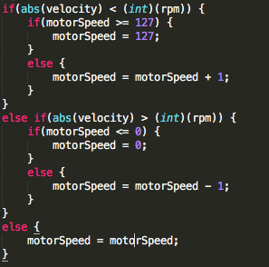
This worked, but it took forever to stabilize. This was due mostly in part to the mass of the flywheel, and the fact that the inertia was messing up the microcontroller. This meant that the motor power would oscillate until it finally got a value that was stable, which is what we wanted, but it did it in 10 seconds, which is something that we did not want (Keep in mind that the whole match is 1.5 minutes long). So we had to work up on another solution.
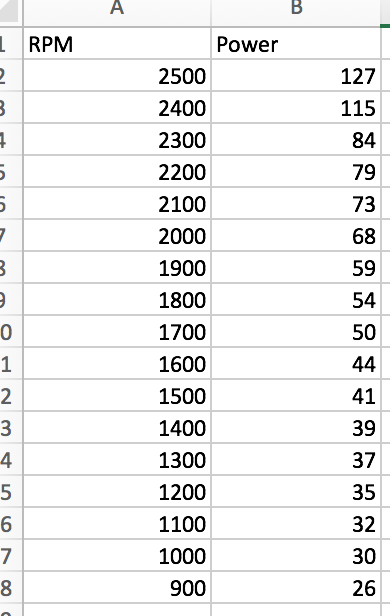
We had the code to determine the motor power for any desired omega, so we decided to just take a bunch of data points and make a function out of it, which we did:
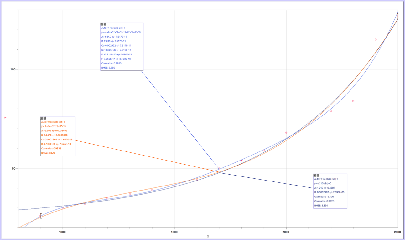
![]()
Now, this worked great, but the problem was that our correlation coefficient wasn’t 1, so we didn’t have an accurate function, at least the precision to what we needed. Then we realized if we combined this function with the oscillation, we would be able to have a accuracy of the oscillator program, with the speed that the function offers. This can be modeled with the following graph:
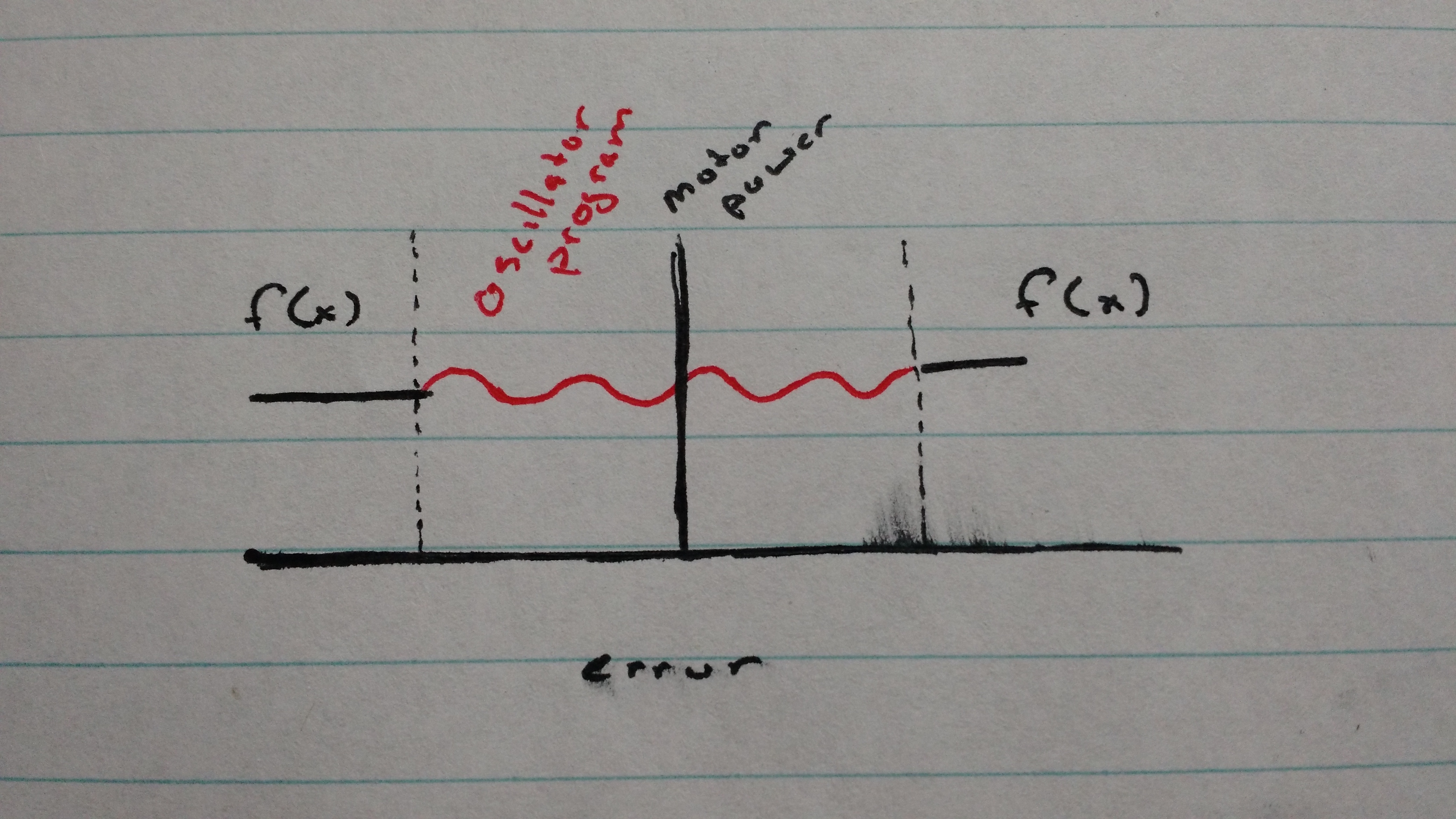
In this case, error = (actual omega – desired omega). Basically when the user changes the desired rpm, the program gets a baseline number (determined by the function above) and uses that until the error gets within a certain threshold (indicated by the dashed lines). Once the error is within that threshold, the oscillation program takes over, and the amount of time that the oscillator takes is reduced because the motor speed is already close enough to the stable value that the oscillator only has to do a minimal amount of work:

This reduced our rev up / recovery time to 2.5s, and got us to worlds! However, I still wasn’t satisfied. Which leads me to *sigh* last night.
What I was thinking was that the function gave a fairly accurate value (which isn’t actually the case, but I’ll elaborate on that later), so I thought, why not use more power the higher the error is to make the recovery time even smaller? That was pretty poorly phrased, so the model below will probably do a better job than I can to explain it:

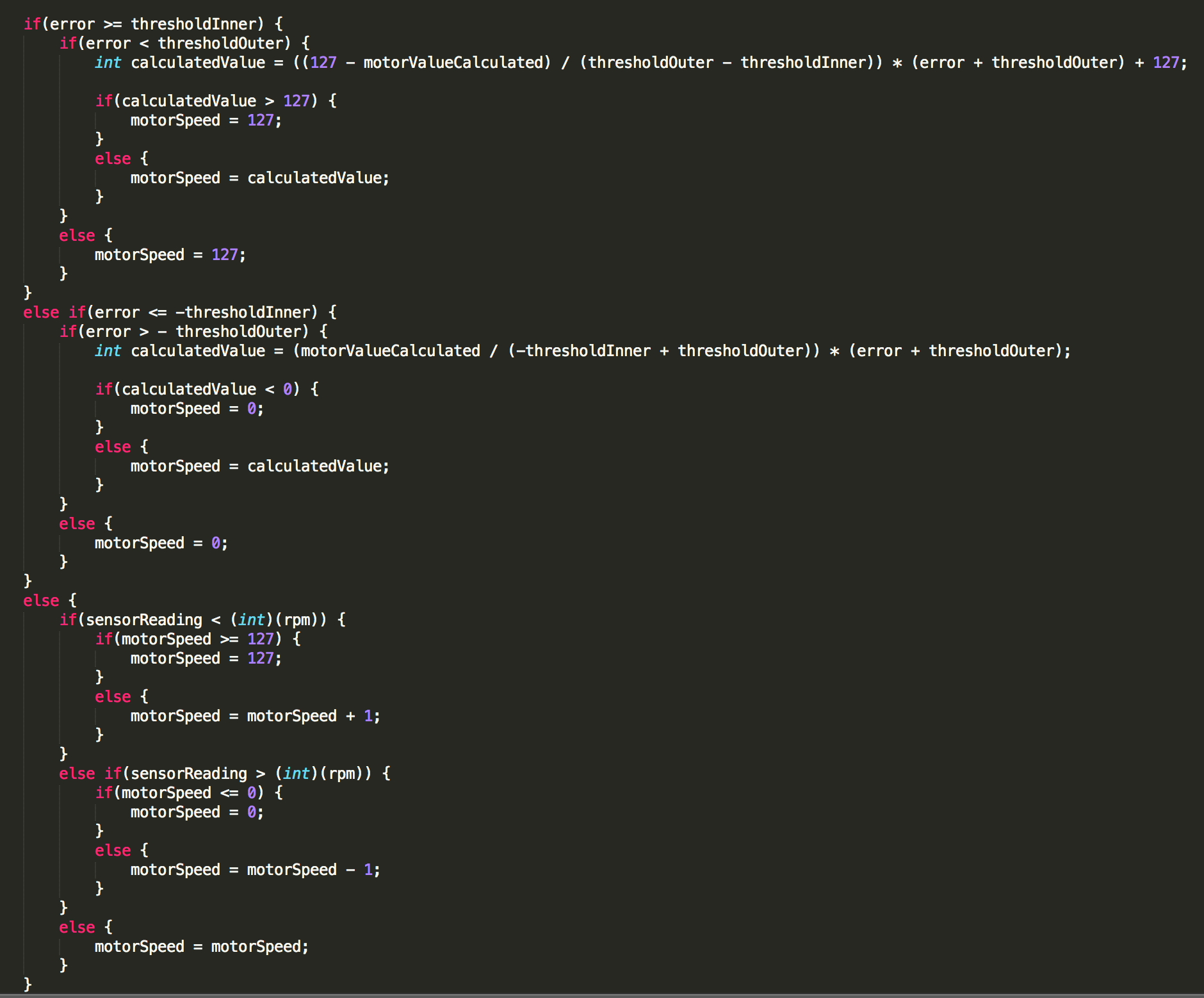
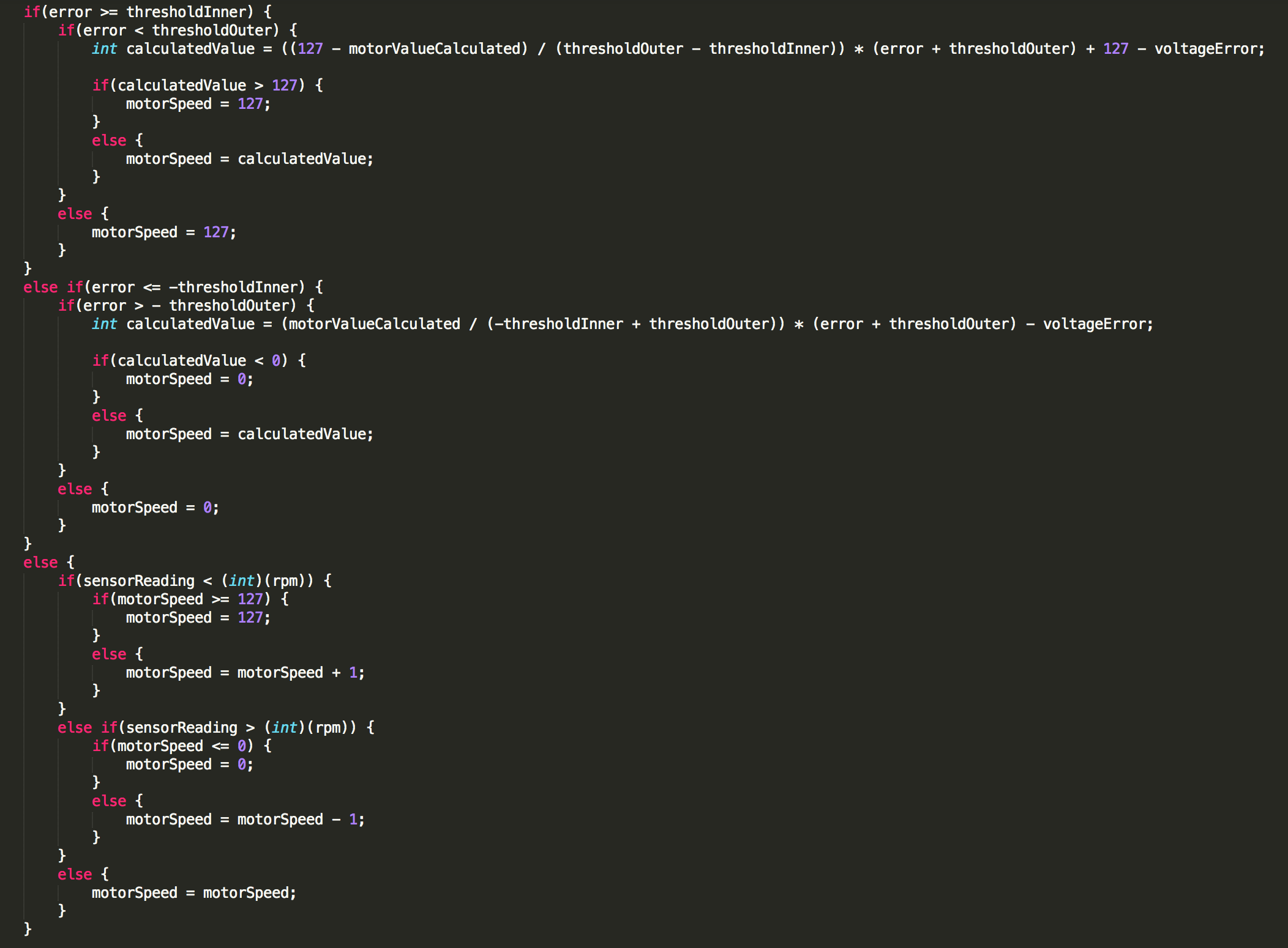
As you can see, the greater the error, the greater or less the motor power, resulting in a derivative with a larger magnitude. It is also important to note that the second point (P2)’s y value is the calculated motor power from the function. What we have there, then is two points, and a linear line that is connecting them. A simple bit of algebra later, and you have the following equations:


Now, this is what you call fast. However, I noticed that there was still a great amount of inaccuracies. After realizing that I was torturing the robot batteries, I realized that the whole function we had was completely reliant on battery voltage.
I connected up a few wires and was able to get a reading of the battery voltages from the microcontroller. I then setup a simple test, where I had a bunch of different voltages and determine the actual motor power required compared to the calculated value:
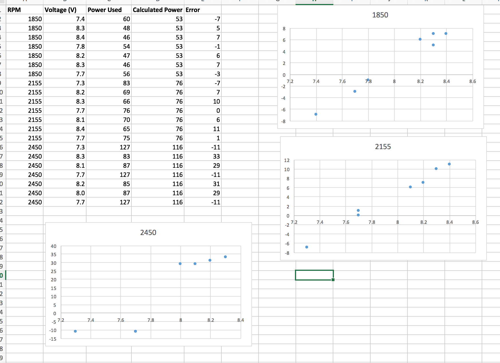
It turns out that the equation for the lines of best fit for the rpms of 1850 and 2155 are nearly the same, and that 2450 starts to plateau off at the end. Instead of making some killer rational function or something like that, I just took the average values from the lines of best fit from the 1850 and the 2155 graphs, and cut it off after the error was over 28 (which was to account for the plateau in the 2450 graph):
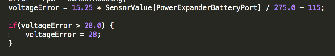
Note: I divided the sensor value by 275 to convert the raw value into volts. After this, I simply offset this value from the other graph:
Now, before the whole internet jumps on me, I now realize that I made a math error that is pretty stupid. Instead of adding an offset to the equation, I should have modified the y value of the point P2 (a couple of images ago) to properly account for the battery error. This was indeed an amateur mistake made at 4 in the morning, however, I came up with a solution that might be able to compensate for that mistake.
So this worked a lot better, however inertia was still a problem. Basically the rate of change of the line was too steep, so the microcontroller couldn’t keep up with the wheel.
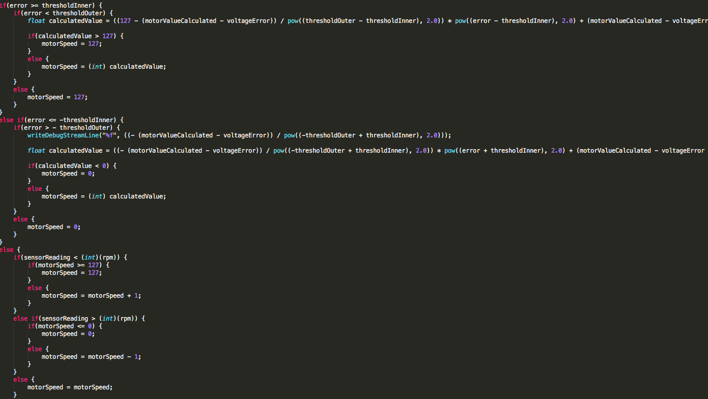
To account for this, I decided instead of using a linear relation between the two points, use a parabolic relationship instead:

After a little algebra: I came up with the following:

After committing it to code (and using the voltage offset on P2, NOT a vertical translation), this is the final result:
And the best part: